Bayesian Changepoint Detection with PyMC3

A client comes to you with this problem:

The coal company I work for is trying to make mining safer. We made some change around 1900 that seemed to improve things, but the records are all archived. Tracking down such old records can be expensive, and it would help a lot if we could narrow the search. Can you tell us what year we should focus on?

Also, it would really help to know this is a real effect, and not just due to random variability - we don't want to waste resources digging up the records if there's not really anything there.

Here's the data:

We could start with some guess of when the change happened, but let's keep this pretty broad. Let's just assume it's was chosen from a uniform distribution from 1860 to 1960.

Assuming there's no foul play involved, it seems safe to assume incidents are independent. And since this is count data, our natural place to start is with a Poisson distribution. We'll have two of these, one on each side of the changepoint. Let's assume these are drawn from the "positive half" of a normal distribution with mean zero and standard deviation 4.

Why not something else? Well sure, there are lots of other choices that could work just fine. the most important thing is that whatever we choose not constrain the distribution any more than needed. Overconstraint can lead to a posterior that "listens" more to you than to the data, while underconstraint can sometimes lead to convergence difficulties. If you "go big" with the prior and it still converges, there's usually no concern.

Back to the model. Given the changepoint and the two means, the count for each year is Poisson-distributed, with mean according to whether the year is before or after the changepoint.

Mathematically, we would write it something like this:

\[ \begin{aligned} T &\sim \text{Uniform}(1860, 1960) \\ \mu_0 &\sim \text{Normal}^+(0,4) \\ \mu_1 &\sim \text{Normal}^+(0,4) \\ n_t &\sim \text{Poisson}(\mu_{[t>T]}) \end{aligned} \]

The \([t>T]\) notation is the Iverson bracket, which is convenient for the situation of a single changepoint (though we'd find something else if we had more than one).

Let's cast this as Poisson regression - independent events, with the event rate changing over time.

Expressing this in PyMC3 is easy:

import PyMC3 as pm

mod = pm.Model()
with mod:
    T = pm.Uniform('changepoint', 1860, 1960)    
    μ = pm.HalfNormal('μ', sd=4, shape=2)
    grp = (coal['date'].values > T) * 1
    y_obs = pm.Normal('y_obs', mu=μ[grp], observed = coal['count'].values)

With the model in hand, we can move ahead to fitting. Since we're doing Bayesian modeling, we won't just find a point estimate (as in MLE or MAP estimation). Rather, we'll sample from the posterior distribution - the distribution of the parameters, given the data.

There are lots of approaches to this, and PyMC3 makes it easy. Let's use slice sampling - for now don't worry too much about why this is a good way to go.

with mod:
    step =  pm.Slice()
    trace = pm.sample(step=step)

Here's a plot of the results.

pm.traceplot(trace);

On the left we have posterior density estimates for each variable; on the right are plots of the results.

PyMC3 samples in multiple chains, or independent processes. Here we used 4 chains. In a good fit, the density estimates across chains should be similar. Ideally, time-dependent plots look like random noise, with very little autocorrelation.

Remember, \(\mu\) is a vector. We have two mean values, one on each side of the changepoint.

We see some interesting bimodality in the changepoint estimate; let's get back to that. Also, the poterior distributions two means are very well-separated. It's almost certain there was a real change in the rate of disasters - it's not just faulty perception on our part.

One thing we might be concerned with is the potential for strong correlations in our posterior estimates. If the changepoint occurred very early, the second group would include some of the higher counts, potentially inflating its mean. This wouldn't necessarily be cause for alarm, but it's something we should be sure to understand.

Let's visualize the dependency, to see if this is the case.

plt.plot(trace['changepoint'], trace['μ'], '.', alpha=0.3)
plt.xlabel('Changepoint')
plt.legend(["Before", "After"])
plt.ylabel('Group means');

We do see some slight dependency. For very early changepoints, the After group is inflated, and for very late changepoints, the Before group is supressed. But the effect appears to be minimal.

plt.hist(np.floor(trace['changepoint']), bins=13, normed=True,align='left');

df = pd.DataFrame({
  'changepoint': trace['changepoint'], 
  'μ0': trace['μ'][:,0], 
  'μ1': trace['μ'][:,1]})

plt.bar(coal['date'], coal['count'], label='count')
plt.xlabel('Year')
plt.ylabel('Incidents')

def pl(pt):
    grp = (coal['date'] > pt['changepoint']) * 1
    line = plt.plot(coal['date'],pt['μ0']* (1 - grp) + pt['μ1'] * grp, 
      color='red', alpha=0.005)    

    
df.apply(pl,axis=1);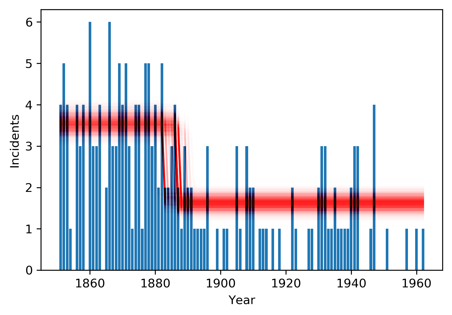

Let's zoom in near the change point:

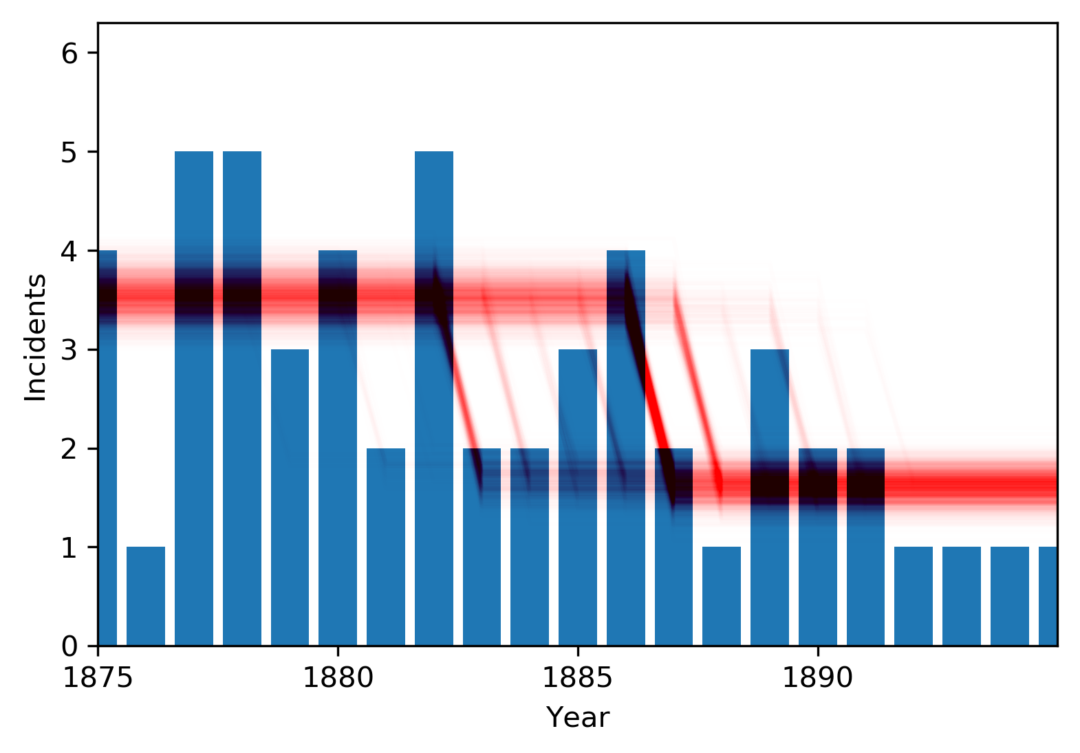
This last plot helps explain the bimodality we were seeing before. Counts in 1885-86 are higher than surrounding years. Maybe the changepoint is just before them, and the higher counts are due to randomness. Or maybe the changepoint is immediately after, and the high counts are because the change has not yet occurred. Either scenario is plausible, though the latter is much more likely.

There's so much beyond this, in PyMC3, other probabilistic programming systems, and Bayesian modeling in general. If you haven't used these methods before, I hope this might give you some glimpse of the power and fexibility of this modeling approach.