Harder Than it Needs to Be
Say you've just fit a (two-class) machine learning classifier, and you'd like to judge how it's doing. This starts out simple: Reality is yes or no, and you predict yes or no. Your model will make some mistakes, which you'd like to characterize.
So you go to Wikipedia, and see this:
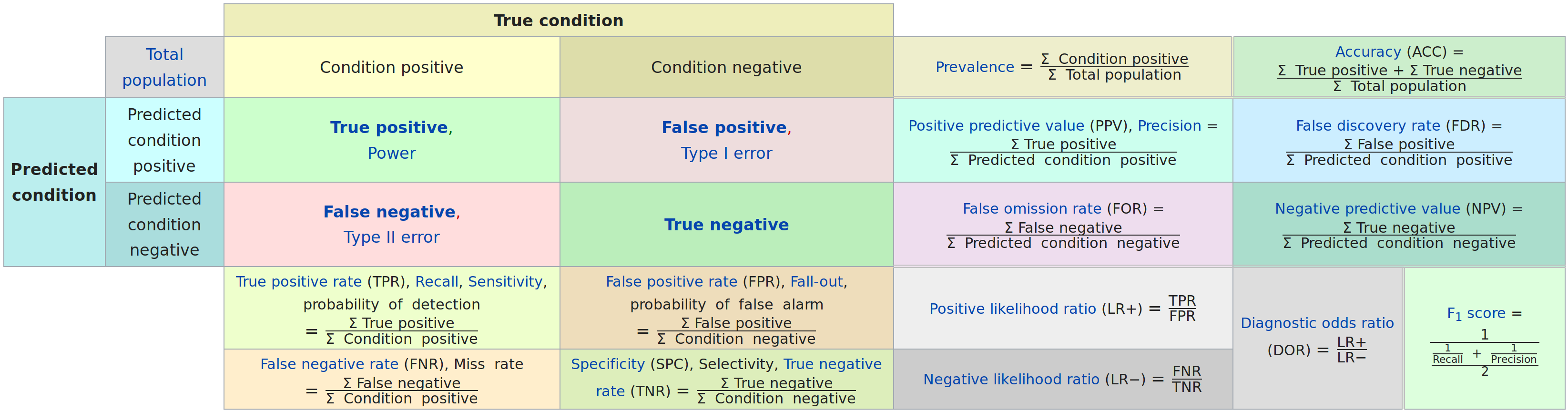
There's a lot of "divide this sum by that sum", without much connection to why we're doing that, or how to interpret the result. Sure, we could click on a given link and read about it, but it all seems a bit more complex than it needs to be.
As it turns out, most of the values we're interested in can be expressed concisely and intuitively in terms of conditional probability.
Let's start with false positive rate. The term itself is has lots of potential for confusion:
- We have to remember that "positive" refers not to ground truth, but to our prediction.
- "False" doesn't mean we predicted false. Instead, it means our prediction is wrong.
- "Rate" means we're interested not in the number of false positives, but in their frequency. The natural question, "relative to what?" is not included in the terminology.
The formula for FPR is
\[ \text{FPR} = \frac{\sum \text{False positive}}{\sum \text{Condition negative}}\ . \]
Better notation
Let's write \(y\) for the observed data, and \(\hat{y}\) for our prediction. And we'll use logical negation notation to indicate "false".
Unraveling the original definition into this, we get simply
\[ \text{FPR} = P(\hat{y}|\lnot y) \]
That is, "The probability we predict true, given that the data indicate false".
Compared to the usual formula, this leads more quickly to ways to calculate the value, "filter for \(y\) false, then take the mean of \(\hat{y}\)". And it makes clear that FPR is conditional on the data, so it's unaffected by changes in the relative class frequencies in the data.
Clearer Computations
This may seem like a minor convenience, but my student Mailei Vargas noticed that biased sampling invalidates some classification metrics, andthe traditional formulation makes it especially difficult to reason about models fit on a balanced sample of a large imbalanced data set.
Suppose you start with a large dataset where \(P(y) = 0.001\), and build a model on a small sample of this \(y_\text{sample}\), where \(P(y_\text{sample})=0.5\). Note that the sampling strategy is heavily biased toward the positive class.
The \(F_1\) score is the harmonic mean of precision and recall. How would you compute it?
Conditional probabilities make this significantly easier to think through.
Recall is \(P(\hat{y}|y)\). Because this is conditional on the observed value, it will be unaffected by the bias of the sampling. Put another way, it's reasonable to assume that \(P(\hat{y}|y) = P(\hat{y}|y_\text{sample})\)
Precision is \(P(y|\hat{y})\). Because we fit the model in terms of \(y_\text{sample}\) instead of \(y\), we can't get to this directly. But it's a conditional probability, so Bayes' Law can help:
\[ P(y|\hat{y}) = \frac {P(\hat{y}|y) P(y)} {P(\hat{y}|y) P(y) + P(\hat{y}|\lnot y) P(\lnot y)}\ . \]
We already have three terms from this:
- \(P(\hat{y}|y)\) is the recall
- \(P(y)\) is the proportion of the positive class in the original data, or 0.001.
- \(P(\lnot y)\) is \(1-P(y)\), or 0.999.
The only thing remaining is to calculate the false discovery rate \(P(\hat{y}|\lnot y)\). This is again conditional on the data, so we can assume \(P(\hat{y}|\lnot y) = P(\hat{y}|\lnot y_\text{sample})\) and calculate this on our sample.
Once we have this, we can calculate the precision \(P(y|\hat{y})\) and find the harmonic mean of that with the recall we computed previously. There's still a bit of arithmetic, but I hope you'll agree that the path is much more clear.
As an aside, note that ROC curves only depend on \(\text{FPR} = P(\hat{y}|\lnot y)\) and \(\text{TPR} = P(\hat{y}| y)\). Both of these are conditional on the true \(y\) values, so ROC, AUC, etc are unaffected by biased sampling (as long as the only bias is relative to \(y\)).
A Rosetta Stone
The Wikipedia article on confusion matrices expresses everything in terms of TP,TN,FP, and FN, where the first letter T or F indicates whether the prediction is correct, and the second letter P or N indicates whether the prediction was positive or negative. Here's a translation into conditional probabilities:
\[ \begin{aligned} \text{TPR} &= \frac{\text{TP}}{\text{TP} + \text{FN}} &&= P(\hat{y}|y) \\ \\ \text{TNR} &= \frac{\text{TN}}{\text{TN} + \text{FP}} &&= P(\lnot \hat{y}|\lnot y) \\ \\ \text{PPV} &= \frac{\text{TP}}{\text{TP} + \text{FP}} &&= P(y|\hat{y}) \\ \\ \text{NPV} &= \frac{\text{TN}}{\text{TN} + \text{FN}} &&= P(\lnot y|\lnot \hat{y}) \\ \\ \text{FNR} &= \frac{\text{FN}}{\text{FN} + \text{TP}} &&= P(\lnot \hat{y}|y) \\ \\ \text{FPR} &= \frac{\text{FP}}{\text{FP} + \text{TN}} &&= P(\hat{y}|\lnot y) \\ \\ \text{FDR} &= \frac{\text{FP}}{\text{FP} + \text{TP}} &&= P(\lnot y|\hat{y}) \\ \\ \text{FOR} &= \frac{\text{FN}}{\text{FN} + \text{TN}} &&= P(y|\lnot \hat{y}) \\ \\ \text{ACC} &= \frac{\text{TP} + \text{TN}}{\text{P} + \text{N}} &&= P(\hat{y} = y) \end{aligned} \]