Pricing is a common problem faced by businesses, and one that can be addressed effectively by Bayesian statistical methods. We'll step through a simple example and build the background necessary to extend get involved with this approach.
Let's start with some hypothetical data. A small company has tried a few different price points (say, one week each) and recorded the demand at each price. We'll abstract away some economic issues in order to focus on the statistical approach. Here's the data:

That middle data point looks like a posisble outlier; we'll come back to that.
For now, let's start with some notation. We'll use \(P\) and \(Q\) to denote price and quantity, respectively. A \(0\) subscript will denote observed data, so we were able to sell \(Q_0\) units when the price was set to \(P_0\).
Building a Model
I'm not an economist, but resources I've seen describing the relationship between \(Q\) and \(P\) are often of the form
\[ Q = a P^c\ . \]
This ignores that \(Q\) is not deterministic, but rather follows a distribution determined by \(P\). For statistical analysis, it makes more sense to write this in terms of a conditional expectation,
\[ \mathbb{E}[Q|P] = a P^c\ . \]
Taking the log of both sides makes this much more familiar:
\[ \log \mathbb{E}[Q|P] = \log a + c \log P\ . \]
The right side is now a linear function of the unknowns \(\log a\) and \(c\), so considering these as parameters gives us a generalized linear model. Conveniently, the reasonable assumption that \(Q\) is discrete and comes from independent unit purchases leads us to a Poisson distribution, which fits well with the log link.
Econometrically, this linear relationship in log-log space corresponds to constant price elasticity. This constant elasticity is just the parameter \(c\), so fitting the model will also give us an estimate of the elasticity.
Expressing this in PyMC3 is straightforward:
import pymc3 as pm
with pm.Model() as m:
    loga = pm.Cauchy('loga',0,5)
    c = pm.Cauchy('c',0,5)
    logμ0 = loga + c * np.log(p0)
    μ0 = pm.Deterministic('μ0',np.exp(logμ0))
    qval = pm.Poisson('q',μ0,observed=q0)
There are a few things about this worth noting...
First, we used very broad Cauchy priors. For complex models, too many degrees of freedom can lead to convergence and interpretability problems, similarly to the indentifiability problems that sometimes happen in maximum likelihood estimation. For a simple case like this, it should be enough to make a note of it, in case we run into trouble.
Next, we expect price elasticity of demand \(c\) to be negative, and we may even have a particular range in mind. For example, it could be reasonable to instead go with something like
negc = pm.HalfNormal('-c',3)We'd then have a minor change to express things in terms of negc.
The μ0 line may seem wordier than expected. Yes, we could have just used
μ0 = a * p0 ** cMaking the linear predictor explicit makes later changes easier, for example if we decided to include variable elasticity. Wrapping the value in Deterministic just means the sampler will save values of μ0 for us. This is a convenience at the cost of additional RAM use, so we'd leave it out for a complex model.
Model fitting and Diagnostics
PyMC3 makes it easy to sample from the posterior:
with m:
    trace = pm.sample()
If all parameters are continuous (as in our case), the default is the No-U-Turn Sampler ("NUTS"). Let's get a summary of the result.
pm.summary(trace)| mean | sd | mc_error | hpd_2.5 | hpd_97.5 | n_eff | Rhat | |
|---|---|---|---|---|---|---|---|
| loga | 9.31 | 1.425 | 0.057 | 6.369 | 12.012 | 509.0 | 1.0024 |
| c | -1.58 | 0.392 | 0.015 | -2.325 | -0.781 | 511.0 | 1.0026 |
| μ0__0 | 51.38 | 5.854 | 0.210 | 40.090 | 63.167 | 660.0 | 1.0013 |
| μ0__1 | 40.11 | 3.145 | 0.089 | 34.211 | 46.619 | 1072.0 | 1.0017 |
| μ0__2 | 32.47 | 2.517 | 0.066 | 27.487 | 37.516 | 1311.0 | 1.0041 |
| μ0__3 | 27.00 | 2.758 | 0.090 | 21.963 | 32.720 | 819.0 | 1.0050 |
| μ0__4 | 22.94 | 3.087 | 0.112 | 17.327 | 29.193 | 660.0 | 1.0050 |
This gives us the posterior mean and standard deviation, along with some other useful information:
mc_errorestimates simulation error by breaking the trace into batches, computing the mean of each batch, and then the standard deviation of these means.hpd_*gives highest posterior density intervals. The 2.5 and 97.5 labels are a bit misleading. There are lots of 95% credible intevals, depending on the relative weights of the left and right tails. The 95% HPD interval is the narrowest among these 95% intervals.n_effgives the effective number of samples. We took 2000 samples, but there are some significant autocorrelations. For example, our samples from the posterior of \(c\) have about as much information as if we had taken 511 independent samples.Rhatis sometimes called the potential scale reduction factor, and gives us a factor by which the variance might be reduced, if our MCMC chains had been longer. It's computed in terms of the variance between chains vs within each chain. Values near 1 are good.
Back to our problem. Results here look pretty good, with the exception of \(n_\text{eff}\).
Let's have a closer look what's going on. Here's the joint posterior of the parameters:
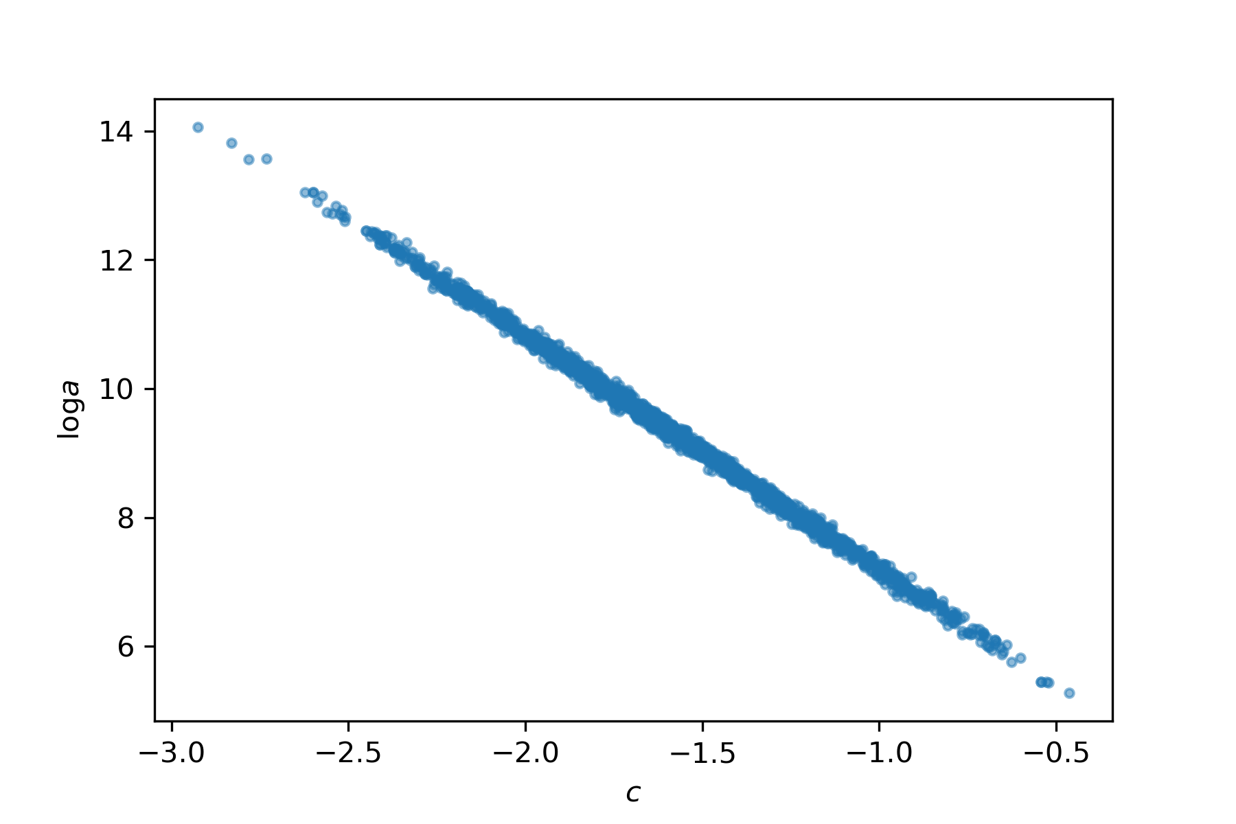
This strong correlation is caused by the data not being centered. All of the \(\log P_0\) values are positive, so any increase in the slope leads to a decrease in the intercept, and vice versa. If you don't see this immediatley, draw an \((x,y)\) cloud of points with positive \(x\), and compare slope and intercept of some lines passing through the cloud.
The correlation doesn't cause too much trouble for NUTS, but it can be a big problem for some other samplers like Gibbs sampling. This is also a case where fast variational inference approximations tend to drastically underestimate the variance.
Just to note, this doesn't mean Bayesian method can't handle correlations. Rather, it's that the representation of the model can have an impact. There are lots of ways of dealing with this, including explicit parameterization of the correlation, as well as several reparameterization tricks. Let's look at a simple one.
Reparameterization
The trouble came from off-center \(\log P_0\) values, so let's try taking that into account in the model. A quick adjustment does the job:
with pm.Model() as m2:
    α = pm.Cauchy('α',0,5)
    β = pm.Cauchy('β',0,5)
    logμ0 = α + β * (np.log(p0) - np.log(p0).mean())
    μ0 = pm.Deterministic('μ0',np.exp(logμ0))
    qval = pm.Poisson('q0',μ0,observed=q0)
Note that we've changed the names of the parameters, to keep things straight. If we wanted to transform between the two parameterizations, we could equate the two logμ0 expressions and solve the system of equations (constant terms equal, and \(\log P_0\) terms equal).
Let's see how it does.
with m2:
    t = pm.sample()
pm.summary(t)| mean | sd | mc_error | hpd_2.5 | hpd_97.5 | n_eff | Rhat | |
|---|---|---|---|---|---|---|---|
| α | 3.49 | 0.080 | 0.002 | 3.335 | 3.640 | 1625.0 | 1.0015 |
| β | -1.73 | 0.411 | 0.010 | -2.530 | -0.937 | 1657.0 | 0.9990 |
| μ0__0 | 52.96 | 6.208 | 0.148 | 41.560 | 65.273 | 1516.0 | 1.0002 |
| μ0__1 | 40.43 | 3.253 | 0.078 | 34.483 | 46.979 | 1346.0 | 1.0014 |
| μ0__2 | 32.10 | 2.614 | 0.061 | 26.667 | 36.777 | 1673.0 | 1.0013 |
| μ0__3 | 26.25 | 2.831 | 0.065 | 20.492 | 31.379 | 1780.0 | 1.0003 |
| μ0__4 | 21.97 | 3.103 | 0.071 | 16.201 | 28.079 | 1758.0 | 0.9998 |
Much better! Note that it's not the parameters that were affected; \(n_\text{eff}\) has also improved for the \(\mu_0\) values, which are directly comparable across models.
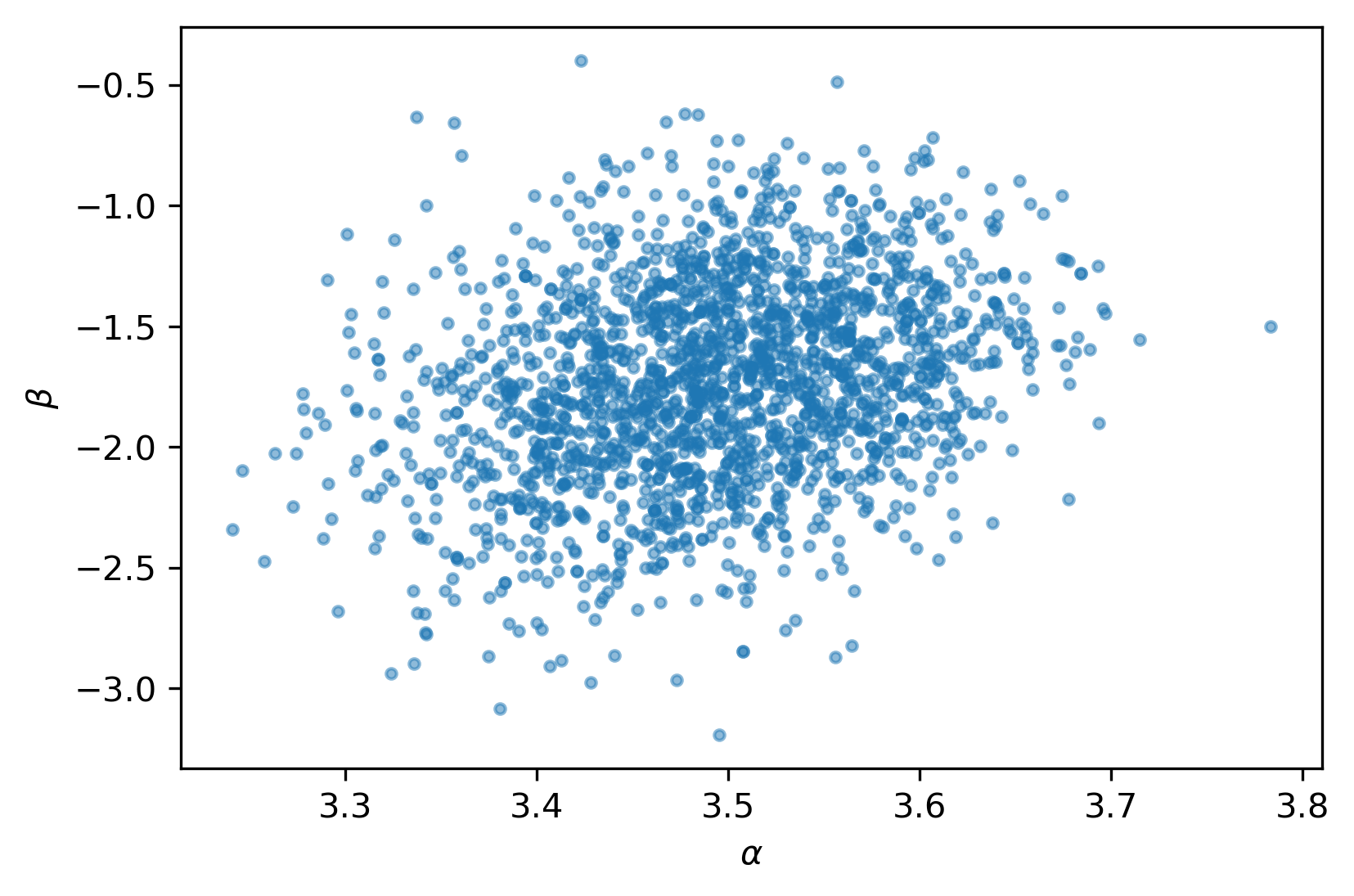
And of course, the parameter correlations are much better:
There are a few other useful tools we can explore. Here's the trace plot:
pm.traceplot(t);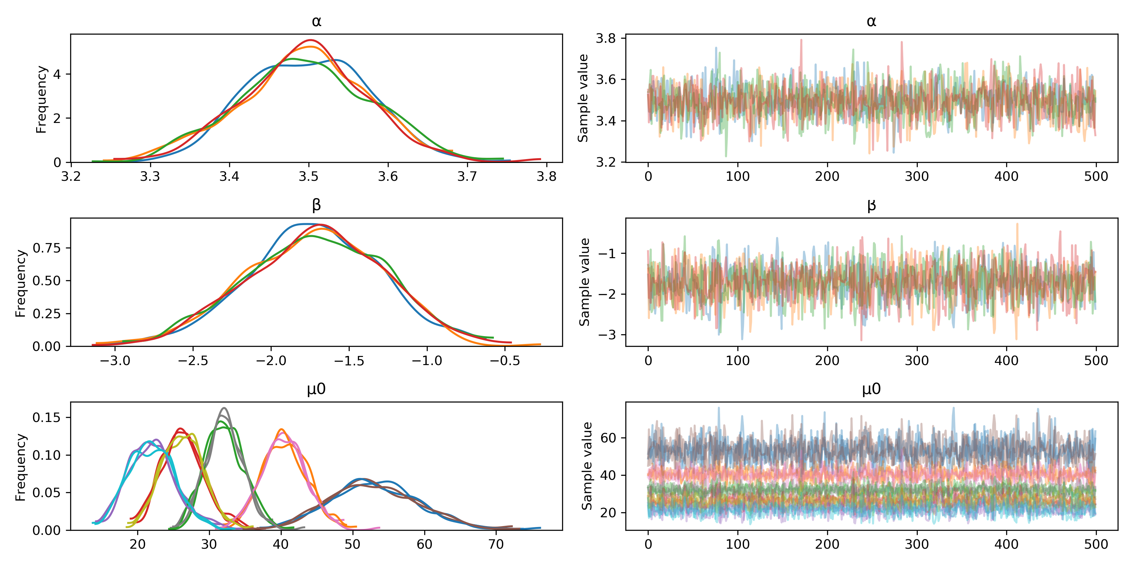
Sampling is done using an independent (Markov) chain for each hardware core (by default, though this can be changed). The trace plot gives us a quick visual check that the chains are behaving well. Ideally, the distributions across chains should look very similar (left column) and have very little autocorrelation (right column). Note that since \(\mu_0\) is a vector, the plots in the bottom row superimpose its five components.
Sometimes we need a more compact form, especially if there are lots of parameters. In this case the forest plot is helpful.
pm.forestplot(t,varnames=['α','β'])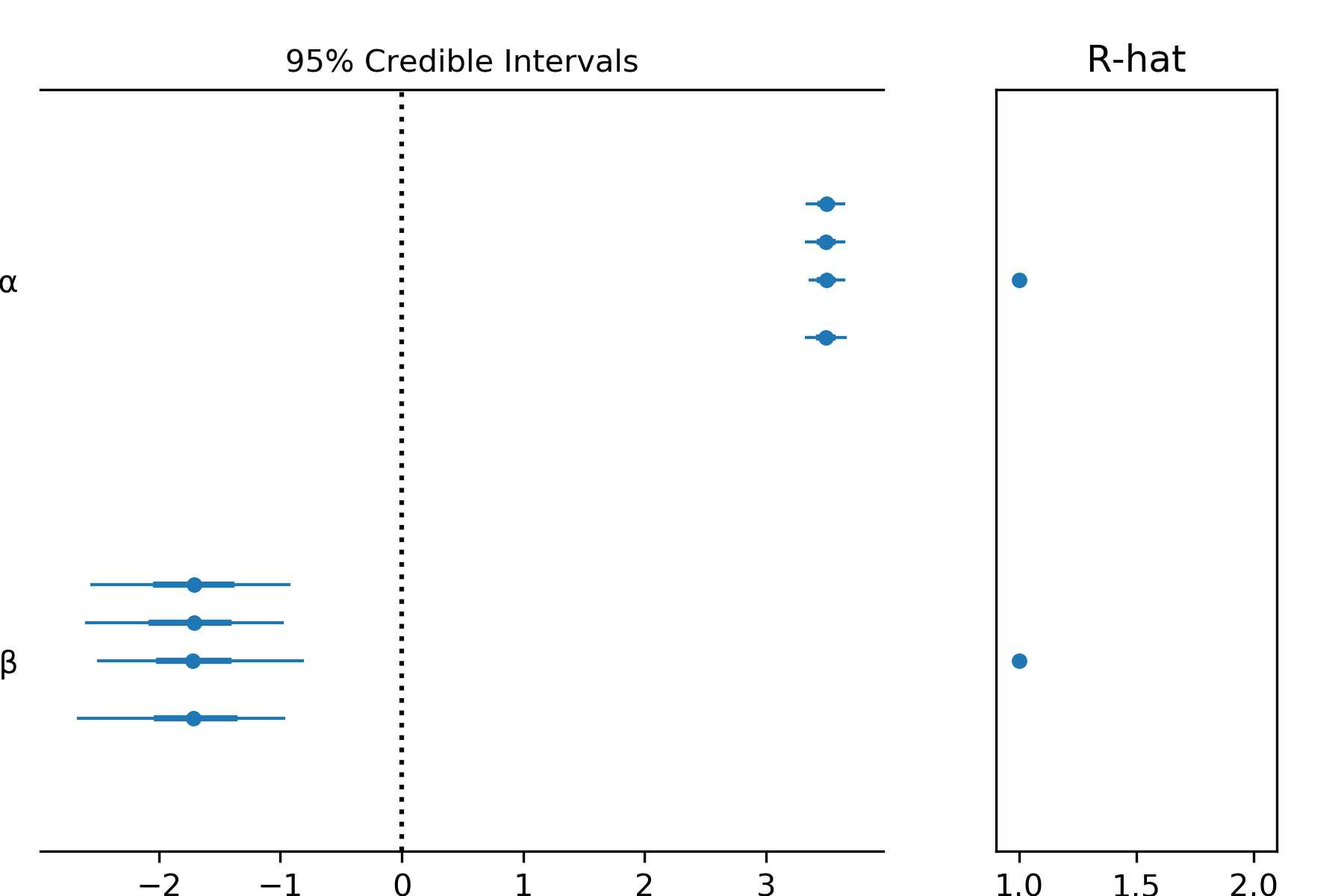
Posterior Predictive Checks
The trace we found is a sample from the joint posterior distribution of the parameters. Instead of a point estimate, we have a sample of "possible worlds" that represent reality. To perform inference, we query each and aggregate the results. So, for example...
p = np.linspace(25,55)
μ = np.exp(t.α + t.β * (np.log(p).reshape(-1,1) - np.log(p0).mean()))
plt.plot(p,μ,c='k',alpha=0.01);
plt.plot(p0,q0,'o',c='C1');
To be concise, I've left out some simple code like axis labels, etc. Here's the result.

Each "hair" represents \(\mathbb{E}[Q|P]\) according to one sample from the posterior. On introducing the data I suggested the point \(P_0=40\) may be an outlier. At first glance, the above plot might seem to confirm this. But remember, this is not a conditional distribution of \((Q|P)\), but of its expectation.
The following boxplot makes this point more explicitly:
plt.boxplot(scipy.stats.poisson.cdf(q0,mu=t['μ0']));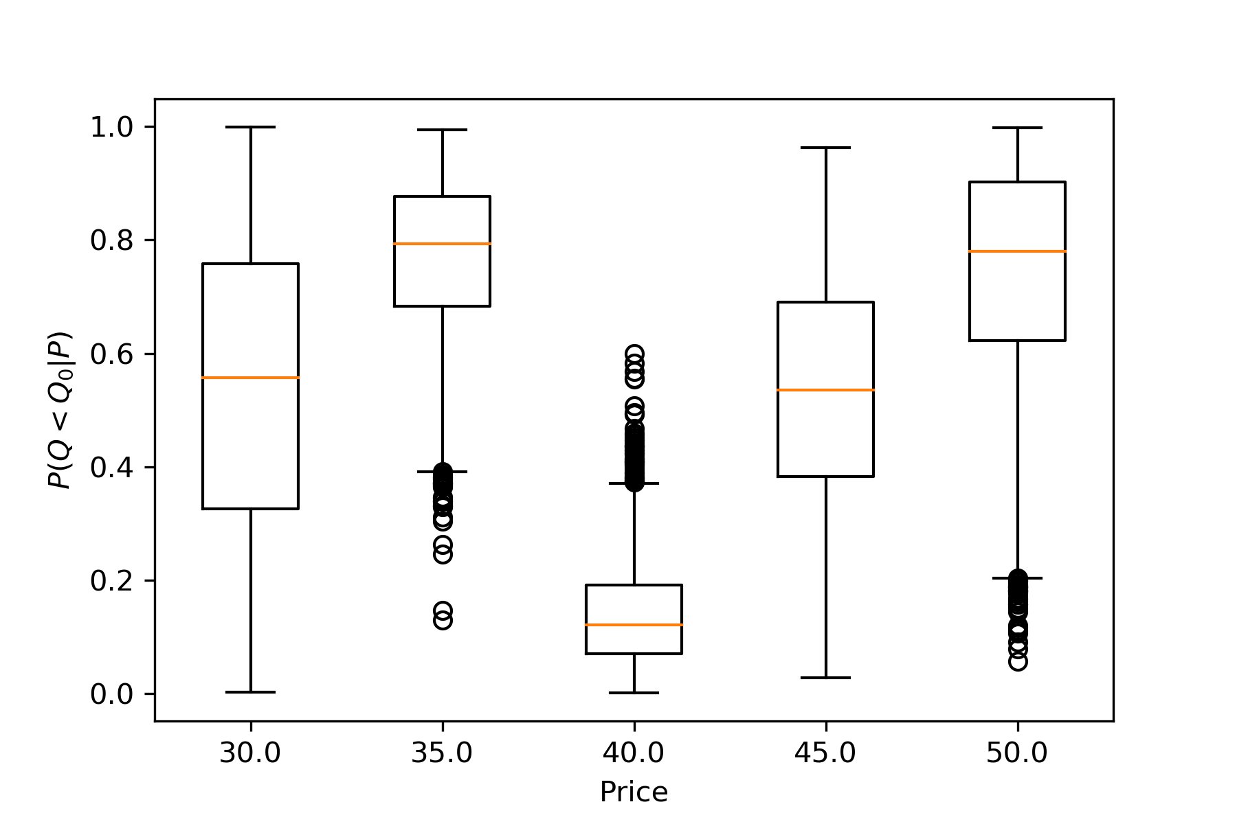
Think of this as asking each possible world, "In your reality, what's the probability of seeing a smaller \(Q\) value than this?" The responses are then aggregated by price. For \(P_0=40\), about half the results are above 0.1. The point is a bit unusual, but hardly an outlier.
This shouldn't be considered a recipe for the way to do posterior predictive checks. There are countless possibilities, and the right approach depends on the problem at hand.
For example, another very common approach is to use the posterior parameter samples to generate a replicated response \(Q_0^\text{rep}\), and then comparing this to the observed response \(Q_0\):
np.mean(q0 > np.random.poisson(t['μ0']), 0)which yields
array([ 0.5055, 0.7265, 0.1055, 0.451 , 0.7 ])
These are sometimes called Bayesian \(p\)-values. For out-of-sample data, results for a well-calibrated model should follow a uniform distribution.
Optimization
We're almost there! Suppose we have a per-unit cost of $20. Then we can calculate the expected profit for each realization:
k = 20
π = (p - k).reshape(-1,1) * μ
With a few array indexing tricks, we can then calculate the price that maximizes the overall expected profit (integrating over all parameters):
plt.plot(p,π,c='k',alpha=0.01);
plt.plot(p,np.mean(π,1).T,c='C1',lw=2,label="$\mathbb{E}[\pi|P]$");
plt.fill_between(p,(np.mean(π,1)-np.std(π,1)).T,(np.mean(π,1)+np.std(π,1)).T,alpha=0.1,color='C1')
plt.plot(p,(np.mean(π,1)+np.std(π,1)).T,c='C1',lw=1,label="$\mathbb{E}[\pi|P]\ \pm$1 sd");
plt.plot(p,(np.mean(π,1)-np.std(π,1)).T,c='C1',lw=1);
pmax = p[np.argmax(np.mean(π,1))]
plt.vlines(pmax,300,900,colors='C0',linestyles='dashed',label="argmax$_P\ \mathbb{E}[\pi|P]$")

plt.ylim(300,900);
plt.xlabel("Price $P$")
plt.ylabel("Profit $\pi$")

plt.legend();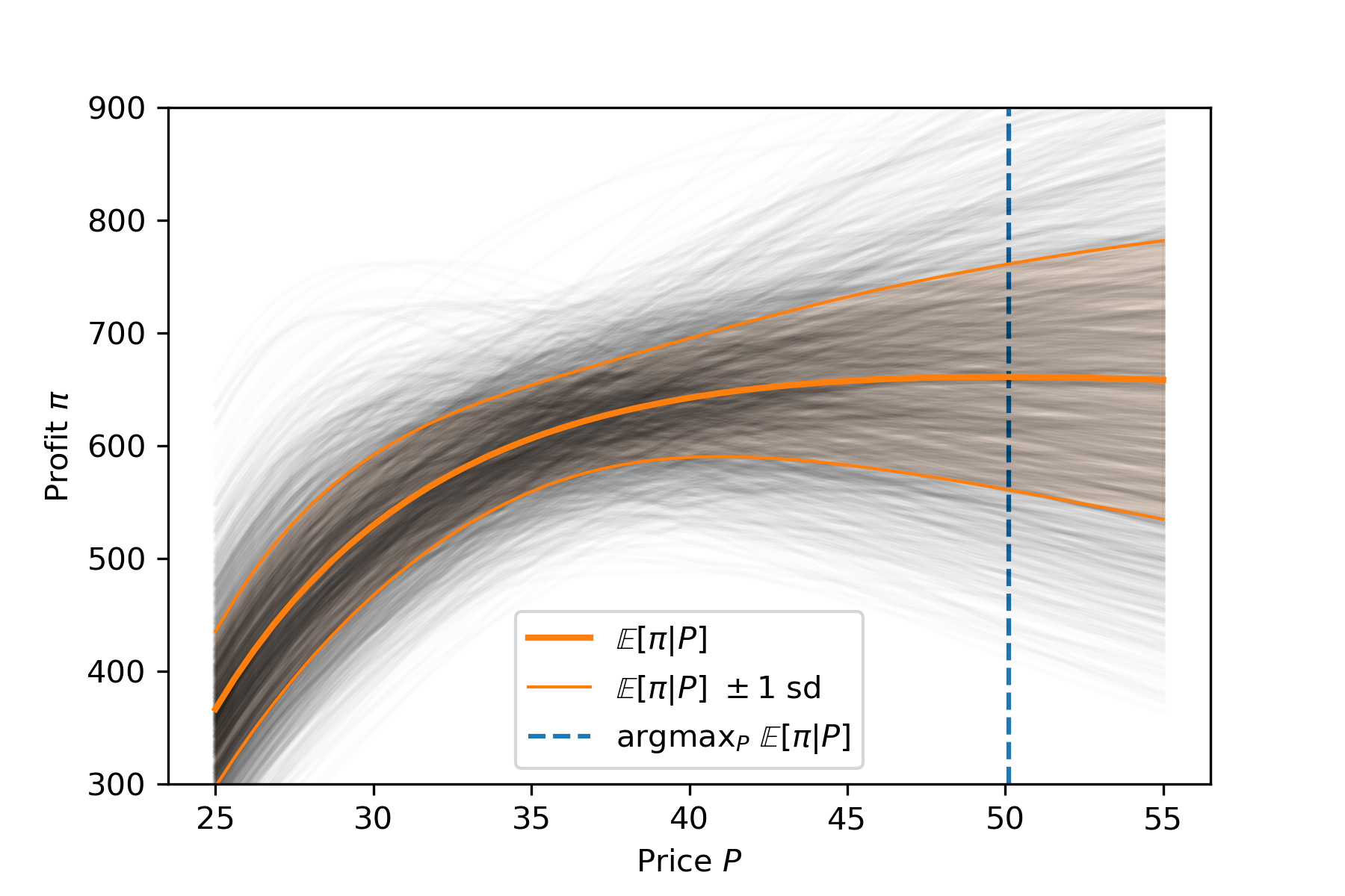
This suggests an optimal price of $49.
Caveats
So... are we done? NO!!! There are some lingering issues that we'll address next time. For example, is expected profit the right thing to maximize? In particular, our estimate is well above the best worst-case scenario (highest unshaded point below the curves). Should we be concerned about this?
Also, the mean is very flat near our solution, suggesting the potential for instability in the solution. Can we quantify this, and does it lead us to a different solution?